The Economic Intuition Behind CBO and JCT Scores

The Congressional Budget Office (CBO) produces about 1,000 cost estimates a year and fulfills thousands more requests from the offices of Members of Congress. This partnership between congressional staff and budget analysts is essential to the legislative process, helping Members understand the fiscal implications of their policy ideas.

Yet Members from both sides of the aisle sometimes find that the final score doesn’t quite capture what was intended. A request to the budget agencies might yield an estimate showing minimal revenue effects when significant behavioral responses were expected, or CBO’s analysis might reflect different implementation assumptions than the Member envisioned.

These surprises often stem from a natural gap between Member offices and agency staff. Most congressional staff aren’t economists, but need to rely on advice from agency staff who have more experience in that field. The economic models that generate budget scores rely on frameworks and assumptions that aren’t well known outside of economics courses. When these assumptions aren’t explicitly discussed upfront, even a clearly written request can lead to analysis that answers a slightly different question from what was intended.

This Fiscal Lab primer translates these economic concepts into practical knowledge for congressional staff. Readers will learn how economists build the models behind budget scores, what assumptions drive their predictions, and which questions will lead to more productive consultations with agency analysts.

With these fundamentals, staff can engage CBO and the Joint Committee on Taxation (JCT) as informed partners by asking sharper questions, clarifying assumptions, and ensuring that technical analysis aligns with legislative intent.

Economic Models Describe How People Make Choices

Economics is the study of how people make choices. People have unlimited wants but limited resources, so they must choose which wants to satisfy. Economic analysis starts from the notion of opportunity cost and making decisions at the margin.

The opportunity cost of a decision is the value of the best alternative not chosen. This is easiest to see with a choice between two alternatives. For example, suppose someone has a choice to see concerts with Eric Clapton or Bob Dylan, who are playing at the same time. If he chooses to see Clapton, he gives up the opportunity to see Dylan.¹

Assuming that people will choose the things that are more valuable over the things that are less valuable, given the resources available leads to a number of predictions. The example above doesn’t place a precise value on the Clapton show, but we know it must be at least as great as the choice to see Dylan.

Often people are confronted with decisions that have more than two choices. In those cases, all options can be ranked from best to worst, and the decision can be reduced to a choice between the best and second-best options. For instance, the choice of how much to work in a week could be any amount of time between zero and 168 hours.

The key element in economic analysis is the choice at the margin—the difference between two options. For someone to work 40 hours in a week, he first must work for 39 hours. Because the first 39 hours of work apply in both choices, they are irrelevant to the decision. The choice depends on the value placed on the last (marginal) hour of work and the opportunity cost of the best alternative use of that hour.
Models are helpful because they are a framework for applying the principles of opportunity cost and marginal thinking to evaluate many possible choices rapidly. Iterating on these small decisions across many possible market conditions builds supply and demand curves.

From Simple Choices to Supply and Demand

Buyers and sellers bring goods to a market to trade. Each buyer or each seller in the market is presented with a choice of what quantity of goods to buy or sell given the market price.

Buyers face a choice at the margin. To get one unit of the good, they must give up the market price. As long as the marginal benefit of buying another unit exceeds the market price, consumers will want to buy another.

Sellers face the opposite choice. To get the market price, they must give up one unit of the good. Conversely, producers will produce as long as the marginal cost of production remains below the market price, which is their marginal benefit.

But in both cases, the optimal choice is made when marginal cost equals marginal benefit.

A single price leads to a single optimal quantity demanded or quantity supplied. Repeating the process for multiple different prices produces supply and demand curves corresponding to multiple different optimal quantities. Figure 1 shows what such a plot looks like.

Figure 1. Market equilibrium

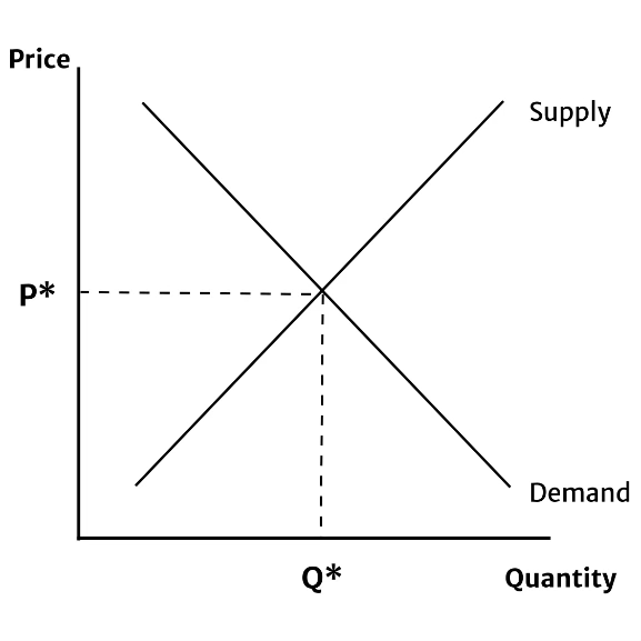
The equilibrium price P* is the price that sets the quantity demanded equal to the quantity supplied at Q*.

Economists draw supply and demand curves on a graph with quantity on the horizontal axis and price on the vertical axis. Supply goes to the sky, indicating that for any given price, sellers will be willing to provide a larger quantity as the good gets more expensive. Conversely, demand curves slope down, showing that as something gets more expensive, consumers wish to buy less of it.

There’s a point on the graph where these two curves cross. If the price is above that, there’s a surplus; the quantity supplied is greater than the quantity demanded. If the price is below that, there is a shortage; the quantity demanded is greater than the quantity supplied. The market price will adjust until it reaches equilibrium where the quantity supplied equals the quantity demanded. Surpluses drive the price down, while shortages drive the price up.

Eventually, the market settles at a price where quantity demanded equals quantity supplied. That price represents a market equilibrium, where outcomes tend to settle. The objective of an economic model is to compute the relevant equilibrium prices and quantities.

Models in Practice Are Built on Supply and Demand

If congressional staff understand the simple model of supply and demand, then they understand the key ideas behind the more complicated models that CBO and JCT use to score bills.

In an introductory economics class, there’s not much more detail than what’s explained above. Students practice analyzing scenarios by figuring out whether an event will shift supply or demand, which direction an event will shift supply and demand, and whether that will tend to raise or lower the market price or increase or decrease the market quantity. Analysis is done with graphs, and simply getting the direction of change is sufficient.

At the intermediate level, students start to add a little more detail. Supply and demand curves are represented with linear equations with the form y = mx + b. The solution to a model involves solving a system of two equations. Often, getting the solution involves algebraically setting the quantity demanded equal to the quantity supplied and finding the price that satisfies the remaining equation.

Figure 2. Parts of an equation of a line

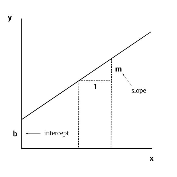
The parameter b determines the y-intercept. Increases (decreases) in b will shift the line up (down). The parameter m determines the slope of the line, or how steep it is. Increases (decreases) in m will make the line more vertical (more horizontal).

At the graduate level and in models used by CBO and JCT, solutions use linear algebra and multivariable calculus to solve systems of many equations. While the math is more complicated, the intuition behind the solution method remains the same.

Different models may have different variables, but all economists ask the same set of questions when building a model:

• How can I use an equation to represent supply and demand?
• How do I solve the equation for the equilibrium market price and market quantity?
• How do different variables in those equations, other than price and quantity, affect the market’s tendency to find a new equilibrium in response to the changes in those variables?

Using Models to Analyze Policy Changes

A model describes the relationships between different concepts. There are often more concepts than the model can predict, so it’s important to divide the concepts into exogenous variables, endogenous variables, and parameters. Exogenous variables are determined outside the model, while endogenous variables are determined within the model. That is, given the exogenous variables, the model makes predictions about the endogenous variables. Parameters are values that are adjusted so that the predictions fit observed data.
For example, there is a relationship between diet, exercise, and body weight. A simple model would predict that changes in body weight are determined by calories consumed by the diet and calories burned through exercise. In this case, diet and exercise are exogenous variables while body weight is an endogenous variable. The model can’t explain whether someone will eat vegetables or a cheeseburger, and it can’t explain whether someone will choose to watch TV or go for a run. But given information about diet and exercise, it can make predictions about changes in body weight. However, different people burn calories at different rates, so the exogenous variables alone don’t necessarily lead to accurate predictions. The model also needs parameter values that capture differences in basal metabolic rates and exercise efficiency. Parameters generalize the model so that it can be adapted to different cases.

Returning to the equation for a line y = mx+b, y and x are the endogenous variables, while the slope m and the intercept b are exogenous. Thus, these are often going to be key factors that influence how a policy gets translated into the ultimate effects on the market.

Fiscal policy variables are frequent examples of polices that shift supply and demand. For example, shifters could be tax rates or spending amounts. From the standpoint of households and firms in the market, they don’t have control over what the government’s policy is. Therefore, any changes in fiscal policy will affect the quantity demanded or supplied for every possible price, resulting in a shift of supply or demand curves.

When staffers make a request of CBO, they should think carefully about the exogenous variables in the model. CBO controls the models that determine the response of the endogenous variables, but the exogenous variables are chosen by Congress.

The supply and demand shifters are the policies that move the intercept. But what’s also important is the slope, which in economics is usually an elasticity. The elasticity measures how much the optimal quantity changes in response to changes in price.

A classic example of this in fiscal policy is labor supply elasticities. Suppose there is a tax cut that raises after-tax income. The tax cut is a change to an exogenous variable that shifts the supply of labor. How much does that increase the quantity of labor supplied? Whether the shift primarily affects the market price or quantity depends on the elasticities of labor supply and labor demand, which are parameters.

Using the right elasticity is critical for making predictions in constructing dynamic scores, or scores that incorporate macroeconomic feedback.² For a tax cut to generate substantial revenue through macroeconomic feedback, there needs to be sufficiently large elasticities to increase the tax base. If the government is taking a smaller slice, it hopes to cut from a bigger pie. Without large elasticities, dynamic scores will not differ much from conventional scores.

There are two main ways to set parameter values. The first is estimation. Estimation involves finding relevant historical data, using the data to fill in values in the model equations, and finding the parameter values that make the model fit the data as closely as possible.

With modern statistical software, it is easy to gather a dataset, perform some calculations, and report a parameter value. The task for economists is to select the right equations so that the estimated parameter values represent the appropriate concept for modeling a policy. A common difficulty with economic data is isolating the effect of a policy while holding everything else constant. For example, data show that the people with college education have higher incomes, suggesting that college raises incomes. However, college attendance is also correlated with other factors that raise incomes, like intelligence. A proper identification strategy shows that economists have taken care to control for confounding variables.

The second way to set parameter values is calibration. A calibrated model has parameter values chosen to match some plausible target value. The target value may come from averages in historical data, or it may come from other parts of the economic literature. For example, CBO’s life-cycle growth model chooses a set of parameters so that certain targets match a benchmark economy similar to the US in recent years.³ These targets include the capital-output ratio, interest rate, Frisch elasticity of working hours, and revenue targets as shares of GDP.

Using Economic Theory to Read CBO Scores Critically

Congressional staff are not professional economists and shouldn’t need to be. However, staff should be informed consumers of CBO reports. When staff receive a report from CBO or JCT, they should ask the following questions:

• Which model was used for the analysis? CBO should be able to explain the intuition and basic steps to derive a solution, even if only at a high level. For instance, if a request asks for a dynamic score with macroeconomic feedback, then one of its macro models should be used.
• What simplifying assumptions go into the model? Every model simplifies reality to make calculations manageable. Check that any simplifying assumptions are plausible and reflect what was requested.
• Did CBO specify the exogenous variables as intended? While CBO writes the models for analysis, Congress chooses the policies to be analyzed. Ensure that there was no miscommunication when policy requests were converted for analysis.
• Do the chosen parameter values match the policy story in the request? For estimated variables, agency staff should be able to explain their identification strategy and how they controlled for confounding variables. For calibrated variables, they should be able to explain why they chose the calibrated value and whether there is a consensus or debate about the appropriate value in the literature.
• How certain are the estimates? Inputs to a model are determined with a statistical margin of error. Forecasts from a model represent one outcome from a range of possible future outcomes. Point estimates reported by CBO and JCT are useful, but need a range of uncertainty for complete context.

CBO’s and JCT’s economic models do not have to remain a black box to congressional staffers. Speaking a little bit of economists’ language enables staff to ask informed questions and work more effectively with agency analysts. When staff and economists speak the same language, the legislative process moves more quickly because communication between Members and agencies is clear. The end result is that Congress has the information it needs to set legislative priorities.