The Fiscal Lab Aggregate Revenue and Expenditure Model (FLARE)

The Congressional Budget Office’s (CBO) baseline is a projection of the single most likely budgetary and economic outcome. CBO’s cost estimates score bills against the change from that single point estimate. In practice, both forecasts and the effects of legislation contain some degree of uncertainty, which is critical information for legislators. However, CBO often does not report that uncertainty when they publish their scores.

For example, the energy credits in the Inflation Reduction Act were initially projected by CBO and the Joint Committee on Taxation (JCT) to cost $271 billion over 10 years.¹ The agencies had to make an estimate for uptake of the program without any historical data, which meant their estimates contained more uncertainty than usual. Uptake of the program turned out to be larger than expected, resulting in revisions to the cost estimate of $1,200 billion over 10 years, over four times the initial estimate.² Had lawmakers received a cost estimate with a quantified range of plausible outcomes, they may have taken additional action to offset the risk of the program being more expensive than expected.

Moreover, CBO’s models contain a great deal of detail, but take a long time to prepare. This can leave its reports out of date with events. For instance, just nine days after CBO released this year’s Budget and Economic Outlook, the Supreme Court struck down tariffs imposed under the International Emergency Economic Powers Act (IEEPA).³ After the ruling, CBO produced a separate estimate stating the tariffs were projected to raise about $2.0 trillion over 10 years, but was unable to update the entire baseline to match the new information.⁴

To help lawmakers address these issues stemming from uncertainty, the Fiscal Lab is developing a budget and economic forecast model to complement CBO’s regular baseline reports. The full name is the Fiscal Lab Aggregate Revenue and Expenditure model, or FLARE for short. The model produces a range of estimates, not just a single forecast. The Fiscal Lab model is transparent and fast, allowing users to quickly iterate on policy ideas and update inputs to keep pace with the latest events.

How Our FLARE Model Works

FLARE consists of a budget model and an economic model paired together. The budget model takes economic conditions as given, applies fiscal policy projections, and calculates aggregate revenues and expenditures for the federal government. The economic model can be run with a path for revenues and expenditures as inputs to produce a conditional forecast for economic variables. Iterating on that process incorporates macroeconomic feedback into the budget estimates. Running the budget model without economic feedback produces a conventional estimate.

The task of the budget model is to reproduce the summary Table 1-1 from CBO’s Budget and Economic Outlook. The primary objects are:

• Revenues
• Mandatory outlays
• Discretionary outlays
• Net interest

The budget model takes four economic series as exogenous inputs:

• Real GDP growth
• Inflation (GDP deflator growth)
• Average interest rate on federal debt
• Population growth

The array of fiscal policy levers is simplified greatly. The set of policy inputs is:

• Average tax rate
• Average mandatory spending per person
• Discretionary spending

Given the exogenous and policy variables, a set of relationships determine the remaining endogenous variables:

• Revenues are the average tax rate times the tax base. In this case, the tax base is nominal GDP.
• Mandatory outlays are the average benefit per person times the population.
• Net interest is the average interest rate on debt times the amount of federal debt outstanding.
• The total deficit is revenues less total outlays. The primary deficit is revenues less outlays excluding net interest.
• The new stock of federal debt is the previous stock of federal debt plus the current period’s total deficit.⁵

Baseline

Users could directly specify a path for each of the policy variables over the entire projection window. However, they can also construct a path by applying simple rules. We include three standard rules to construct a policy path:

1. Current policy. Congress takes every action to keep current policy in place. Tax rates remain constant. Benefit levels and discretionary funding remain constant in real terms, only growing with inflation.
2. Current law. Congress takes no further action whatsoever. Tax rates expire according to schedule. Mandatory programs with dedicated funding sources stop spending when funding runs out. Discretionary funding runs out at the end of the current fiscal year.
3. Present baseline rules. Applies the rules as written in Section 257 of the Deficit Control Act.⁶ Congress takes some reasonably expected actions, but stops short of keeping all current policy in place. Tax rates expire as scheduled. Mandatory spending continues as written, regardless of funding. Discretionary spending grows with inflation.

Economic Model

The economic model is a Bayesian Vector Autoregression (BVAR).⁷ We use six variables—the four exogenous variables from the budget model plus aggregate revenues and outlays.

The model predicts future values of the six series based on past values of each of the six series. It captures the interrelationships between the series based on how they move together.

The key aspect of the BVAR is that it incorporates uncertainty into the model. It contains two types of uncertainty:

• Uncertainty about future events. Rather than project a smooth path, the model draws multiple realistic paths and averages over them. The result is not just a point estimate of the most likely path, but an entire distribution of potential future paths.
• Uncertainty about model parameters. One common way to specify small models is to calibrate their values to match historical data. The Bayesian approach generalizes that process. It starts by specifying a distribution of prior beliefs about the parameter values, then updates the distribution given observed data. Where calibration sets exact parameter values, the Bayesian approach considers multiple parameter values at once if that is consistent with the data.

Forecast

Taken together, the BVAR and budget model produce outcomes that are quite close to CBO’s baseline despite using less information and simpler modeling.⁸

Figure 1. Budget forecast 

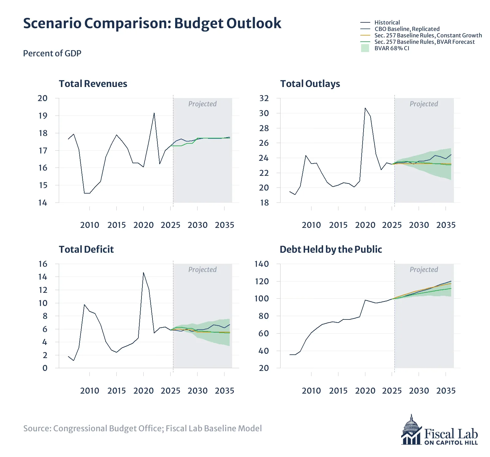
Figure 1. Scenario comparison of the budget outlook: total revenues, total outlays, total deficit, and debt held by the public as a percent of GDP.

Figure 1 shows the budget forecast.

• Revenues. Revenues are specified as a share of GDP, so by definition that ratio does not vary. Our simplified input matches CBO in the back half of the budget window.
• Outlays. The BVAR closely tracks a constant growth rate. CBO’s baseline shows outlays growing as a share of GDP later in the budget window, but still within the BVAR forecast’s credible interval. Consequently, the deficit projection looks similar.
• Debt Held by the Public. The constant growth rate is close to CBO’s baseline. The BVAR projects lower debt-to-GDP ratios, driven mainly by a faster growth projection, which is discussed in the next section.

Figure 2. Economic forecast 

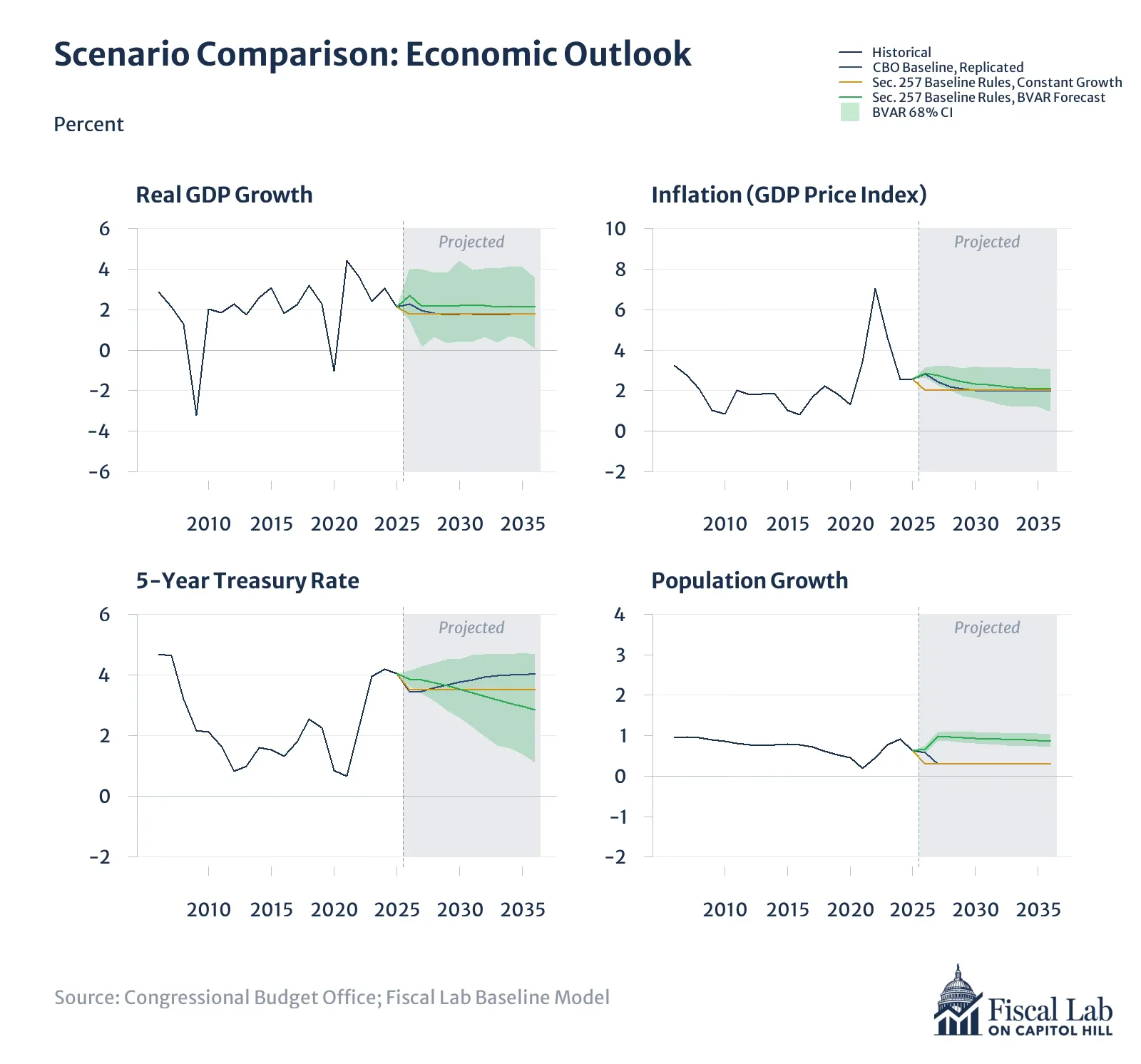
Figure 2. Scenario comparison of the economic outlook: real GDP growth, inflation, the five-year Treasury rate, and population growth.

Figure 2 shows the economic forecast.

• Real GDP. CBO’s baseline closely hews to a constant growth rate of 1.8 percent per year, while the BVAR expects growth to average slightly higher. Again, the forecast bounds and variation in the historical data show that the projections are still close together.
• Inflation. Both CBO’s baseline and the BVAR forecast converge to an inflation rate of 2.0 percent per year, though the BVAR expects inflation to remain elevated for a longer period of time. All three forecasts are within the BVAR credible interval.
• Interest rates. Interest rates in the BVAR show a drop back toward historical averages. However, the CBO baseline expects rates to remain constant or increase slightly as federal debt levels remain elevated and increase risk premia for bond holders. Yet, the BVAR recognizes that rates can change quickly and produces forecast bounds that include the CBO baseline.
• Population. Population is the biggest divergence between CBO’s baseline and the BVAR. The BVAR predicts that population growth returns closer to the historical average. It lacks additional information like the population structure and the history of fertility rates that could improve projections of near-term population changes.

Planned Development

This Brief is a research preview of a model still in development. We will add additional features over the next few months. Our top priorities are:

• Additional detail. The current output works directly with aggregate accounts. The next step is to create projections down to more detailed levels and sum them up to get aggregate totals. Outlays can be broken down by function, and further down to the individual account level. Revenues can be broken down by type of revenue stream. More economic data series can go into the BVAR to provide additional forecast information. Additionally, a cohort-component demographic model would add more detail to the population projections affecting mandatory spending and labor markets.
• Growth model core. The BVAR model expects the future to look similar to the past. This is fine when the economy will return to its previous growth path. However, many major reforms could move the economy to a different growth path entirely. Specifying potential output as a function of capital stock, labor force, and productivity would allow policy that affects capital stock and labor force to shift the growth path. Then shifting the BVAR to model the output gap instead of real GDP directly converts the BVAR to a model of the fluctuations around the growth path.⁹
• Hierarchical forecasts. Many of the series that we are interested in forecasting share a relationship where one series is the sum of component series. That relationship provides additional information that could be used to improve the forecast and tighten the forecast bounds.¹⁰
• Stochastic volatility. A key feature of the BVAR is the shocks that capture unmodeled and uncertain events. Macroeconomic series tend to display periods where changes are larger than other periods, as seen recently in the Global Financial Crisis and Covid-19 pandemic. Stochastic volatility relaxes the assumption that period-to-period changes have the same distribution at each point in time, which allows the model to capture the periods of calm and periods of crisis seen in economic data.¹¹ We are eager to expand this feature of the BVAR. 
• Interactivity. We want to be transparent, so that users can see the simplifications and assumptions that allow the model to be tractable. There is both an art and a science to modeling. Where parameter choices fall within the realm of art, we alert the user and allow them to make different choices if they desire.

We welcome feedback from congressional Members, staff, and public policy experts as we continue to develop this baseline model.